The most recent project in my Udacity nanodegree gave me a 6 jointed robot arm and a desired path for the robot's gripper. My job was to perform the inverse kinematic analysis to calculate the joint positions that will move the gripper along the requested path. After learning the forward kinematics and doing a full geometric analysis for the inverse kinematics, my robot arm was able to follow the paths it received with negligible error.
Denavit–Hartenberg Analysis
A single free body in space requires definition of 6 variables to define its position, and most commonly used are x, y, z, roll, pitch, and yaw. Standard spacial translation and rotation matrices can be used to fully define a system with 6 degrees of freedom, but this would mean each 4x4 transform matrix would involve 6 variables for each joint location. Because every transform matrix is multiplied together to complete the forward kinematic analysis, the computations required rapidly become complex.
The Denavit–Hartenberg (DH) parameters were developed to cut down the variables required at each joint from 6 to 4, thus lowering the overall computation time. Microprocessors everywhere breathed a sigh of relief. A high level outline of this method is shown below.
To use this method I sketched the robot arm and determined axis orientation based on the parameters:
Built a table of parameters based on the sketch and additional geometry information:
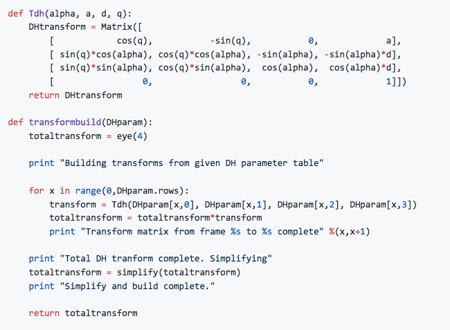
And built some functions to compile the required transformation matrix
That allowed me to piece together the forward kinematics so I could calculate where in 3D space the robot's gripper was located and oriented based only on the joint positions.
Inverse Kinematics
The inverse kinematics is used to calculate the joint positions after receiving a position and orientation of the robot's gripper. A full discussion of this requires its own report, but I can offer the following summary of the steps required:
- Calculate the x,y,z position of Joint 5
- Use a hearty helping of the law of cos alongside arctan to calculate the first three joint positions using only the x,y,z found in step 1.
- Apply knowledge of Euler's angles and rotation matrices to perform a separate analysis to find the last three joint positions.
- Pray that you didn't flub any rotations or misunderstand the orientations required.
- Shove some inverse kinematic code into the ROS server and hope it works
Udacity left the students to figure out most of this informationon on their own for this project, which led to a lot of discussion in the community Slack as everyone struggled to debug together. After my own share of failed attempts, it was time to try a full test of the project.
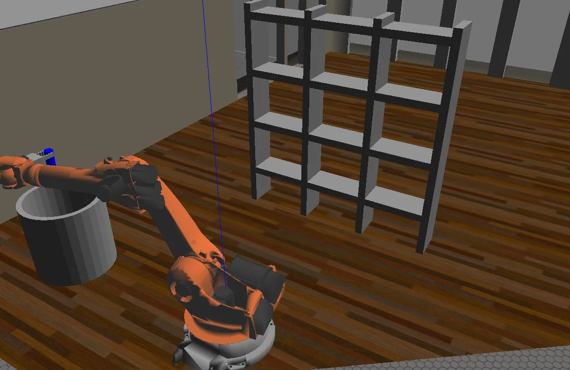
Grabbing target can
Dropping target can
Success! My arm is picking and grabbing from all locations with ease! Well, with as much ease as the Udacity provided virtual machine could muster on my Macbook Air. Robot Operating System (ROS) only functions on Linux, and Udacity will only offer official support for their provided VM. I've read about some painful experiences other students have gone through to get projects running on a native Ubuntu install, so I'm sticking with the slower VM for the moment.
At this point my project met all the required criteria for submittal, so I turned it in and received my congratulatory code review the next morning. Except...I decided to go a little deeper.
Error checking
While working on my analysis I was logging the cartesian distance between the path point requested and the path point my code returned. This ensured my forward kinematics and inverse kinematics matched, and it was super helpful for late stage debugging.
After submitting, I decided to refresh my limited experience with matplotlib and started building some plots to visualize the path and how much error I was getting.
Moving from neutral position to grab can
Moving from shelf to trash can after grabbing can.
Let's take a closer look at another path:
I made these plots for 15 different paths and saw similar error ranges in each. The displacement error observed is hitting exactly where we expect typical floating point error to show up, showing that my math was performing as advertised.
Trends
I'm not well versed in the details of floating point precision and rounding error, so I wanted to see if any robot orientations were consistently producing high error. I was concerned that there would be some near singularities for certain joint angles that don't play well with arctan.
The following two graphs were compiled to check for patterns of higher error.
No angles or positions seem to jump out as concerning, so it looks like my joint orientations worked out fairly well for this analysis.
Conclusion
All in all, this shows that my code is running geometry calculations that produce the requested values with a very high degree of accuracy. If the real world application did not require precision to 10^-15, there are a variety of optimization options that would speed up the calculations but potentially increase error. The analysis tools I've built allow quick comparisons between inverse kinematic methods that may use different tools.
A few of the potential paths forward if I were continuing this project:
- Include orientation (roll/pitch/yaw) in the error calculation
- Build a new Inverse Kinematics server that uses more rounding to decrease calculation time.
- Observe the effect of using
chop = Trueon SymPy's evalf function. - Log the computation time for each calculation
- Compare the floating point error between SymPy (used for the matrix multiplication here) and NumPy.


