“I wrote this report for a class called Vehicle Communication Systems while in pursuit of my M.S. at The University of Tulsa. The internal network of a car is fascinating, and I hope this serves as a half decent introduction to some of the concepts. This project was my first steps into the world of python, and it’s been my language of choice since.”
1. Introduction
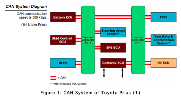
As cars become more and more complex with the addition of components that have the ability to record data, the communication between these systems becomes more and more important. CAN is now standard on any new car sold in the United States. Hybrid vehicles are becoming more common as consumers value fuel efficiency more with the rising price of gas. The Toyota Prius is currently the highest selling hybrid vehicle and it will be used in this project to observe the connection between the vehicle’s CAN data and the real world. The components seen on the Prius’ CAN may be seen in Figure 1.
Seen in Figure 2 is the typical HUD of the Prius. The average fuel economy for every 5 minute chunk of time is presented to the user, along with a live mileage bar that updates every second. This report will be primarily focusing on obtaining the mileage values displayed.
2. Procedure
This project used a VSI-2534 manufactured by Dearborn Group to connect to the Toyota Prius. A variety of data was produced and analyzed to produce readable engineering data. This process is described in the following sections.
2.1 Connection to Vehicle
Dearborn Group provides a program called DLM2 alongside the VSI-2534. This software allows capturing raw data files of the CAN bus traffic. The VSI connects to the OBDII port on the Prius and to the laptop via a USB cable. The VSI is pictured in Figure 3.
Once the drivers are and DLM2 are installed on the computer, the device must be configured in the software’s “device configuration” window, seen in Figure 4. The connected device appears in the “J2534 devices” section and the detected channels are read through use of the “Get Info” button. A channel is selected and a .dbc file can optionally be associated with this channel. Associating a .dbc file allows the user to view the translated engineering values in the RX window in real time but does nothing to the raw log file.
2.2 Data Generation
After the device is connected and the channel configuration applied, the computer will begin to receive messages from the bus once the start button is pressed. The messages are viewed live in a receive window, and display filters can be set up if a .dbc file is used. Once a receive window is open and recording, the data output can be generated by right clicking the receive window and selecting ‘save’. A file is selected and messages are appended to it until the ‘save’ button is clicked again.
For this project, a variety of data logs were generated, and multiple tests were run with VBox gps data being transmitted onto the hub at the same time. This allowed validation of all speed information.
3. Results
3.1 Reverse Engineering CAN IDs
Using the DLM2 software and observation of the live data a number of CAN IDs were identified. Table 1: CAN ID DefinitionsTable contains values that were able to be physically corroborated through car interaction and observation of the DLM2 receive window.
For values related to other components of the system, such as battery and fuel information, research done by Atilla Vass was used. A compilation of his theories on the CAN IDs was used to determine the correct direction to head in when plotting mileage data (3).
3.2 Python Code
To generate plots, a python script was written that generates a plot from a raw text file produced from the DLM2 software. A .csv input file is used to determine what CAN IDs to plot and how to translate their values to engineering units. This .csv value acts similarly to a .dbc file whose function is described in the earlier introduction section. The .csv file contains the name of the desired value, CAN ID, conversion factor, length, and location of the data. An example of this input file can be found in Appendix B, while the base code to plot simple values can be found in Appendix A. More in depth calculations were required for fuel economy analysis, and the additional code for this is found in Appendix C.
3.3 Wheel Speed Analysis
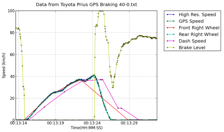
Figure 5, Figure 6, and Figure 7 plot three of the more interesting data files collected. They all contain wheel speed information, GPS speed from the VBox, and two overall speed values found on the bus. Figure 6 also shows brake level information. More plots can be found in Appendix D.
3.4 Fuel Analysis
In Figure 8 fuel economy is plotted from a 5 minute long test. During the test a video camera and timer were used to generate the trip MPG values from the HUD. The live MPG value was generated using a fuel injector value found on the bus along with the high resolution speed. This value was determined through the following formula:
4. Discussion
4.1 DLM2 Timer Issues
While running the 5 minute tests to gather fuel efficiency data, it was noted that the timestamps logged by the DLM2 did not match up with real life expected values. Figure 9 shows this mapped against values broadcast by the VBox. Python was used to find the slope of this line for 8 different data logs. The values ranged from .868 to .887, with an average value of .878. This average slope value was used to correct data generated on further plots by multiplying the DLM2 timestamps by the inverse of the average slope: 1.1388.
4.2 Wheel Speed Analysis
The most notable point seen in the speed plots is the lagging of the dashboard speed. It’s consistently running behind all the other speed values. It has a lower resolution due to only being contained in one byte of data which clearly has an influence. It also appears to be rounded up, likely because that’s the safer choice to present the driver.
The GPS speed closely matched the value given by the vehicle’s front right wheel, generally staying within .25 km/h of it. This is because it was physically closest to this wheel, and it signifies that the vehicle is calibrated well to its wheel speeds. When going in a straight line, the speed values for all 4 wheels would be within .25 km/h, although it was noted that the front axle wheels were either set to broadcast less frequently or had a lower priority on the bus.
4.3 Fuel Consumption Analysis
Overall, the values pulled from the HUD match the overall rising trend seen in the calculated values, but there is enough of a difference to suggest a notable error in calculations. Because the fuel consumption required combining two values that don’t share a CAN ID in a formula, an averaging algorithm had to be used. This took each fuel injector value one at a time and averaged all the previous speed values to use in the equation mentioned in section 3.4.
To plot the running average, the code simply took the average of the all previous values. An issue with this method may be that the frequency of the calculated values varied over time and skewed the average towards sections that had a higher frequency. In the future an integration method should likely be used.
5. Conclusions
·Using DLM2 with the VSI-2534 requires timestamp modification as those written to log files are not accurate and are created at approximately 87.8% the speed of real time.
·The speed displayed to the user on the HUD display lags behind the vehicle’s actual speed.
·Wheel speeds on the bus stayed within .5 km/h of the value recorded by the VBox, indicating strong calibration.
·Fuel economy data calculated through bus values does not match HUD data. The averaging system is the most likely source of error.
6. Future Work
·The python plotting script does not work if the desired data is not contained in full bytes. Rewriting it to read data by bit location would be useful.
·DG has supplied example C++ code to interface with the car through the VSI using SAE’s J2534 standard. Transforming this into a python program was begun but not finished.
7. Works Cited
1. Toyota. Toyota Hybrid System - Course 071. [PDF] Toyota Technical Training.
2. Society of Automotive Engineers. Recommended Practice for Pass-Thru Vehicle Programming. s.l. : SAE, 2004. J2534.
3. Vass, Atilla. The Hybrid 2004 Toyota Prius - My CAN Project. Vass Family. [Online] October 31, 2008. [Cited: February 12, 2013.] http://www.vassfamily.net/ToyotaPrius/CAN/cindex.html.
Appendix A: Python code
import datetime


#data log and faux .dbc file; possibly build an file selector later?
filename='GPS Braking 50-0.txt'
translator='TranslateSpeedBrake.txt'

textfile=open('Data/%s' %filename, 'r')
datalines=textfile.readlines()
textfile.close()

DLCs={} #Data length Code Dictionary that will be used to find all IDs.
timeList=[] #store the timestamp from the log file
IDList=[] #store the IDs in sequence
rawData=[] #Store the data fields in sequence

for line in datalines[8:]: #iterate through the entire file starting at line 8
    elements=line.split() #Separate the entries

    s = elements[1]

    new = s[:12] + s[13:]
    times=datetime.datetime.strptime(new, "%H:%M:%S:%f")

    #adjustment for time offset
    if len(timeList) == 0:
        initialTime=times
    times=(times-initialTime).total_seconds()*1.388

    timeList.append(times)


    ID=elements[0] #extract the text associated with the CAN identifier
    IDList.append(ID) #add the ID to a list

    DLC=elements[3] #The DLC text field has a colon, so separate the label from the text
    DLCs[ID]=DLC #Store the DLC in a dictionary with the ID as a key. This will ensure only unique IDs are used as keys.

    Datalength=4+int(DLC)

    rawData.append(elements[4:Datalength]) #store the data field as a list of text strings

IDs=DLCs.keys() #the keys in the DLCs dictionary are all the unique IDs that have not been duplicated.


print('Number of Unique IDs: %i' %len(IDs)) #display the total number of messages

#Get data from faux .dbc file (currently a .csv produced by hand)
textfile=open('Translators/%s' %translator, 'r')
legend=textfile.readlines()
textfile.close()

xaxis=[]
yaxis=[]

import matplotlib.pyplot as plt


f1=plt.figure(1)

#build time and engineering data for each requested value
for line in legend[1:]:

    elements=line.split(',')
    time=[]
    processed=[]
    raw=[]
    yaxis.append(elements[0])
    xaxis.append('time'+elements[0])

    #build time list
    for i in range(len(IDList)):
        if IDList[i] in [elements[1]]:
            time.append(timeList[i])
            raw.append(rawData[i])

    vars()['time'+elements[0]]=time

    #Turn Raw CAN bytes into engineering units
    #Currently reads byte location from faux .dbc file, future iterations should base from bit location
    for line in raw:
        hexdata=""

        #reads length of data and concatinates hex bytes
        for x in range(0,int(elements[3])):
            hexdata+=line[int(elements[4+x])]

        conversion=int(hexdata,16)*float(elements[2])
        processed.append(conversion)

    vars()[elements[0]]=processed
    plt.plot(time, processed, marker='o', linestyle='-',markersize=3)
    #plt.plot(time, processed, 'o')

plt.xlabel('Time (seconds)')
plt.ylabel('Speed (km/h)')
plt.legend(yaxis,bbox_to_anchor=(1.05, 1), loc=2, borderaxespad=0.)
plt.grid()
ttl=plt.title('Data from Toyota Prius %s' %filename)
ttl.set_y(1.03) #pushes the title up as to not crowd the axis labels
plt.savefig('Plots/%s.png' %filename[:-4],dpi=100,transparent=False, bbox_inches='tight', pad_inches=0.05)
Appendix B: Example .csv input file
Data Name,CAN ID,Conversion Factor,Length of Data, Data Location
High Res. Speed,B4,.01,2,5,6
GPS Speed,302,0.01852,2,4,5
Front Right Wheel,B1,.01,2,0,1
Rear Right Wheel,B3,.01,2,0,1
Dash Speed,3CA,1,1,2
Brake Level,30,.787,1,4
Appendix B: PYTHON CODE ADDITION TO PLOT FUEL ECONOMY
timeIndex = 0
speedtimeindex=0
timeMPG=[]
MPG=[]
averageSpeedBuffer = []
averageFuelBuffer = []
averageMPG = []
timeAverageMPG = []


tenSecond=0
tenSecondCount=timeMpgHUD[tenSecond]

for q in range(len(zippedFuel)):

    while zippedFuel[q][0] >= zippedSpeed[speedtimeindex][0]:
        averageSpeedBuffer.append(zippedSpeed[speedtimeindex][1])
        speedtimeindex=speedtimeindex+1
        #print str(q) +' '+ str(speedtimeindex)

    averagespeed=sum(averageSpeedBuffer)/len(averageSpeedBuffer)

    timeMPG.append(zippedFuel[q][0])

    initialMPG = (10000*averagespeed)/zippedFuel[q][1]

    #Display only reaches 99.9 mpg
    if initialMPG == inf or initialMPG > 99:
        initialMPG = 99

    MPG.append(initialMPG)

    if tenSecondCount < timeMPG[q]:
        averageMPG.append(sum(MPG[70:],dtype=np.int32)/len(MPG[70:]))


        if tenSecond < len(timeMpgHUD):
            tenSecond=tenSecond+1
            if tenSecond < len(timeMpgHUD):
                tenSecondCount=timeMpgHUD[tenSecond]
            else:
                tenSecondCount=inf


    #Only empty buffer if it's not empty
    if not averageSpeedBuffer:
        averageSpeedBuffer = []


plt.plot(timeMPG, MPG, marker='o', linestyle='-',markersize=3)
plt.plot(timeMpgHUD, averageMPG, marker='o', linestyle='-',markersize=3)
Appendix C: ADDITIONAL PLOTS


